Theoretical Overview

Larvaworld is an open-source Python package and virtual laboratory for Drosophila melanogaster larval behavior. It combines agent-based modeling (ABM) with multiscale neural control and supports analysis of both simulated and experimental motion-tracking data. Virtual larvae are implemented as 2D agents capable of realistic locomotion, guided by multimodal sensory input and optionally constrained by a Dynamic Energy Budget (DEB) model that regulates the exploration – exploitation balance according to metabolic needs across the larval life stage.

The platform was developed to address two central challenges in behavioral neuroscience and computational modeling. First, it provides a shared “virtual laboratory” in which experimental data analysis and behavioral modeling are integrated within the same software environment. Experimental locomotion datasets can be imported and converted into a standardized format that is identical to the format generated by simulations, while all derived kinematic and behavioral metrics are computed within Larvaworld using transparent, configurable analysis pipelines. This ensures that simulated and experimental datasets share the same structure and can be analyzed with identical, unbiased methods.

Second, Larvaworld aims to bridge a long-standing gap in theory building between sub-individual models in neuroscience and supra-individual models in ecology. It focuses on the behaving individual as the central modeling unit and explicitly links fast neural dynamics, closed-loop behavior, and slower energetic and life-history processes. Simulations can span sub-millisecond neuronal timescales, sub-second behavioral control, and circadian-scale metabolic regulation, within environments that reproduce established experimental protocols of larval behavioral neuroscience assays.

The design of Larvaworld follows four overarching aims:

• Integration of established theoretical and modeling principles (ABM, DEB, layered behavioral control, modern motion-tracking analysis),

• User-friendliness for both behavioral modeling and data analysis,

• Modularity and extensibility at all architectural levels (models, environments, experiments, analysis),

• Computational efficiency and storage management for large-scale and long-running simulations.

Figure (Sakagiannis et al., 2025) provides a schematic overview of the architectural components and how they interact within the platform. In the remainder of this section we follow that architecture block by block, covering larva models, larva groups, environments, setup and agent-based simulation, data collection and larva datasets, visualization and experiment replay, analysis and model evaluation, and genetic algorithm (GA) optimization. The subsequent pages of the documentation complement this conceptual tour with practical, step-by-step guides, tutorials and API references for installing Larvaworld, running experiments, importing data and extending the platform.

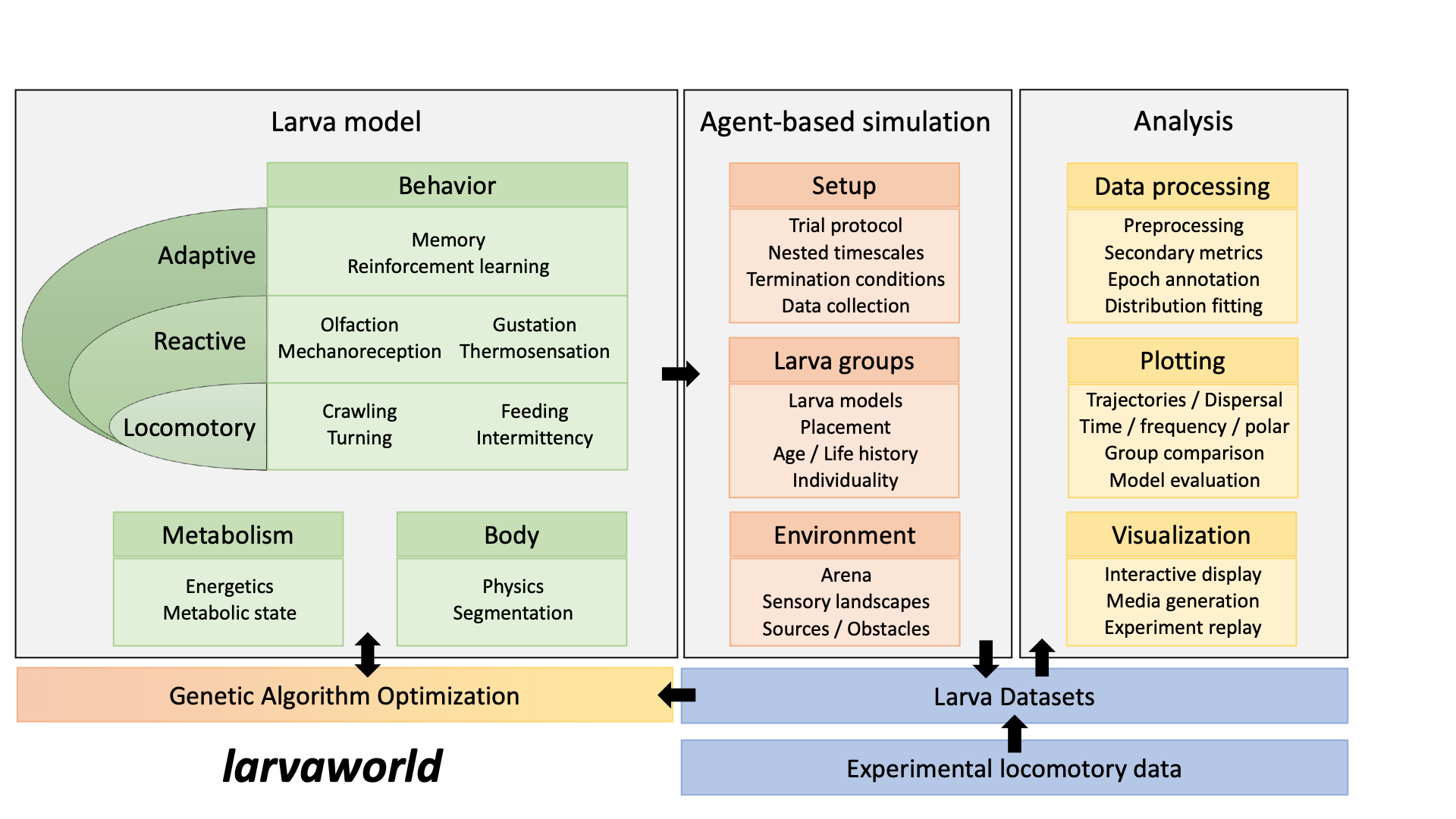
Figure: Schematic of the main components and functionalities of Larvaworld (Sakagiannis et al., 2025).

Larva Model

The Larva model block in Figure represents the virtual agent at the heart of Larvaworld: a single larva with a simulated body, sensory modalities and layered behavioral control.

Body, physics and metabolism

The body is modeled as a simplified 2D structure with one or more segments, supporting:

• realistic locomotion with detailed body midline and contour compatible with common tracking setups,

• optional multi-segment physics for detailed body–arena interactions, simulated in the Box2D physics engine, and

• visualization and analysis pipelines identical to those applied to tracked real animals.

Metabolism and energetics are captured by a Dynamic Energy Budget (DEB) model that runs in the background at a configurable timescale. The DEB model:

• accounts for post-hatch age, rearing substrate and periods of food deprivation,

• reproduces realistic growth curves (body length, wet weight, time to pupation), and

• generates an energetically regulates behavior via a dynamic hunger satiety drive.

This energetic feedback mechanism regulates the exploration–exploitation balance and enables discrete foraging phenotypes such as rovers and sitters through differential configuration of nutrient absorption parameters.

For background on DEB theory, see Kooijman (2010), Dynamic Energy Budget theory for metabolic organisation; for implementation details, see Larva Agent Architecture.

Sensory modalities

Olfaction, mechanoreception, and thermosensation are explicitly represented in the architecture. Sensors are placed at defined body locations (e.g. the head region) and track simulated sensory landscapes:

• Odorscapes generated by odor sources,

• Thermoscapes representing temperature gradients, and

• Windscapes representing airflow and wind direction.

These sensory channels provide the inputs for chemotaxis, thermotaxis, anemotaxis and more generally stimulus-dependent modulation of locomotion. The modular framework makes it straightforward to add new sensory modalities (e.g. visual or hydrosensory cues) by subclassing Sensor.

For sensor configuration, see Brain Module Architecture.

Behavioral Architecture

Behavioral control is organized in three layers, following the subsumption behavioral control paradigm used in behavior-based neurorobotics. The behavioral architecture is introduced in (Sakagiannis et al., 2025)

1. Locomotory layer

Generates the basic motor primitives: crawling, lateral bending and feeding. These behaviors are optionally implemented as oscillatory processes (crawl oscillator, lateral oscillator, feeding oscillator) that can operate independently, interfere or be coupled.

This layer is semi-autonomous: evidence from isolated CNS preparations shows that simple behavioral primitives can be generated even when separated from higher-order control.

2. Reactive layer

Integrates sensory inputs from the environment (e.g. olfactory, mechanosensory) and modulates locomotion based on incoming stimuli. Typical examples include:

• chemotaxis toward or away from odor sources,

• local search in the vicinity of a target,

• contact-triggered reorientations,

• thermotaxis, and

• anemotaxis.

3. Adaptive layer

Hosts slower experience-based processes such as learning. This layer can include memory modules, implemented as reinforcement learning or neuron-level spiking models (e.g mushroom body circuit for olfactory associative learning)

Each layer follows the subsumption principle: top-down modulation from higher layers influences only a few key parameters in lower layers, reflecting subtle adjustments by higher neural centers rather than complete overriding of lower-level control.

Modular, hybrid and extensible design

Each control layer is composed of interconnected modules, specialized for processing specific sensory inputs, generating motor outputs or performing modulatory sensorimotor integration. This toolkit-like, modular design:

• offers a high degree of configurability, enabling researchers to compare models by adding, removing or replacing modules

• facilitates expansion through the seamless integration of new modules, and

• imposes minimal constraints on the modeling detail within individual modules.

Modules can be:

• deterministic or stochastic,

• rule-based, equation-based,

• rate-coded neural, or neuron-level spiking models (Nengo, Brian2),

as long as they conform to standardized input–output interfaces.

This hybrid nature allows neuropile-specific models that lack motor components to be embedded within Larvaworld’s behavioral output framework, and enables direct comparison of competing hypotheses for the same behavioral domain (e.g. different chemotaxis strategies).

For architectural diagrams and runtime interactions, see Module Interaction and Brain Module Architecture.

Larva Groups

The Larva groups block in Figure 1 represents how individual larva models are instantiated into groups with shared traits, reflecting the structure of real behavioral experiments.

Group definition and placement

Virtual larvae are generated in groups, each characterized by:

• the number of individuals,

• a spatial distribution for initial positions, defined by center, scale, shape (e.g. uniform disk, Gaussian cloud) and placement within that shape,

• a range of initial body orientations, and

• group-specific visual and odor identifiers (color, odor signature).

These parameters capture how real experiments are structured—for example, different genotypes or experimental conditions placed at defined arena locations.

For configuration examples, see the tutorials on Single Experiments.

Age, life history and energetics

Each simulated larva group can be associated with a life history: the DEB model is run forward to a chosen age on a defined rearing substrate, including possible starvation or partial deprivation periods. The resulting energetic state (energy reserve density, structural volume, maturity, etc.) is used as the initial condition of the metabolic model when the behavioral simulation starts.

This decouples the rearing phase (typically 3 days for third-instar larvae) from the behavioral assay phase (typically minutes to hours) and allows systematic exploration of how developmental and nutritional history shapes behavior.

Individuality and parameter sampling

Groups can be linked to real experimental reference datasets from which parameters are sampled. The sampling mode controls individuality and variability, with options to:

• optimize for an “average” individual (mean or median parameter values),

• preserve inter-individual variability by sampling sets of parameters from empirical distributions, or

• replicate the reference dataset on an individual-by-individual basis for selected parameters (e.g. match each simulated larva’s crawling frequency to a specific tracked larva).

This supports controlled experiments on individuality and variability, as detailed in the Results section of the companion paper.

For dataset import and sampling workflows, see Reference Datasets.

Environment

The Environment block includes the arena, sensory landscapes and sources/obstacles, defining the virtual space in which larvae move and interact.

Arena

The simulation environment is a 2D arena with configurable geometry (e.g. circular Petri dishes, rectangular arenas, or custom shapes) and boundaries. This matches typical behavioral setups and provides the spatial scaffold for sources, obstacles and sensory gradients.

Arena boundaries can be:

• impassable (larvae cannot cross),

• torus-wrapped (larvae that leave one edge reappear at the opposite edge), or

• open (larvae can leave the arena).

For arena configuration, see Arenas and Substrates.

Sensory landscapes and sources

Sensory landscapes consist of:

• Odorscapes generated by odor sources (simple Gaussian gradients or plumes generated via a diffusion-algorithm),

• Thermoscapes representing temperature gradients, and

• Windscapes representing airflow (configurable air-puffs) and wind direction.

Using diffusable odorscapes within windy environments creates dynamic real-world conditions as odorants are carried by wind createing plumes.

Users can adjust:

• the position and intensity of sensory sources,

• the spatial distribution of gradients (e.g. diffusion coefficient, gradient extend),

• the arena boundaries,

• any internal obstacles (e.g. walls, compartments).

Multiple odor sources with different valences can coexist, enabling preference tests, associative learning assays and navigation tasks.

Substrates and food distributions

Food and odor sources are characterized by:

• substrate type (e.g. standard medium, cornmeal, PED-tracker, sucrose-based),

• nutritional quality (compound densities: yeast, sucrose, agar, etc.), and

• available amount of food.

Substrate can be:

• uniform (distributed over the entire arena),

• arranged as one or more patches, or

• stored in a grid where each cell holds a consumable amount that depletes over time as larvae feed.

Substrate type and quality defines the external food density (or substrate concentration) in the environment, denoted as X in DEB. This affects the larva’s energy assimilation according to a number of DEB parameters like ingestion efficiency, determining how feeding rate translates into energy reserve gain. This enables realistic foraging simulations where larvae grow, mature and modulate their behavior based on feeding history.

For substrate definitions and nutritional parameters, see Table 3 in the companion paper and Arenas and Substrates.

Setup and Agent-Based Simulation

The Setup and Agent-based simulation blocks in the Figure describe how larva models, larva groups and environments are combined into a concrete virtual experiment and how the simulation is executed.

Agent-based backbone

Larvaworld uses an agent-based modeling (ABM) approach built on the agentpy library. Core Model, Space and Object classes are adapted to support nested-dictionary parameterization and modular biological agents.

ABM provides:

• flexible control over agent scheduling (simultaneous or sequential updates),

• clear separation between agents and environment, and

• efficient turn-based data retrieval for time-series recording.

For architectural details, see the “Agent-based modeling” subsection in the companion paper and Simulation Modes.

Trial protocol, timescales and termination

A trial protocol specifies:

• initial conditions (environment, larva groups, life history),

• behavioral and energetic timescales,

• duration or termination conditions (e.g. time limit, larvae reaching a goal), and

• which data and analyses to run.

Larvaworld supports nested timescales:

• Fast neural or synaptic processes (e.g. a spiking MB) at sub-millisecond resolution (e.g. 0.1 ms),

• Behavioral control at sub-second resolution (default 0.1 s), and

• Energetics simulated as a background DEB metabolic model running at longer, even circadian, timestep.

These processes run in parallel, allowing slow developmental and energetic constraints to regulate fast sensorimotor behavior. This multi-timescale approach is depicted in the “Timescales” panel of the paper.

Larva Datasets and Data Collection

The Larva Datasets block in the Figure covers how data are collected during simulations and how experimental locomotion data are integrated into the same standardized format.

Standardized dataset structure

Both simulated and experimental data are stored as LarvaDataset instances, with three core elements:

1. Time-series data A double-indexed Pandas DataFrame (timestep × larva ID) with:

   • primary tracked coordinates: centroid, midline, contour points,

   • derived parameters added during processing: angular metrics, spatial metrics, odorscape navigation metrics, etc.

2. Endpoint metrics A per-larva DataFrame (indexed by larva ID) with summary metrics computed at the end of a simulation or recording (e.g. total distance, mean velocity, dispersion, bout statistics).

3. Metadata A nested dictionary describing experimental conditions, tracking settings, animal groups and storage paths.

DataFrames are stored in HDF5 files under different keys (e.g. midline, contour, trajectory), and metadata are stored in an accompanying configuration file. Datasets can optionally be registered as reference datasets under a unique ID for reuse in optimization, evaluation and batch runs.

For storage and retrieval workflows, see Data Processing.

Experimental locomotory data

Larvaworld imports tracked datasets from several lab-specific formats, including:

• Schleyer lab (12-point midline, constant framerate),

• Jovanic lab (11-point midline, variable framerate),

• Berni lab (single-point, low frame rate, suitable for light-weight long recordings),

• Arguello lab (FIM tracker, configurable spatiotemporal resolution).

Each format has its own framerate and midline/contour resolution. Conversion functions map these formats into the standardized LarvaDataset structure.

Only primary coordinates are imported; all secondary metrics (angular velocity, path length, bout annotations, etc.) are computed within Larvaworld to ensure transparent, reproducible comparisons across datasets.

For import workflows and supported formats, see Lab-Specific Data Import and Table 7 in the companion paper.

Visualization and Experiment Replay

The Visualization block in the Figure comprises interactive display, media generation and experiment replay, enabling real-time inspection and post-hoc visualization of both simulated and experimental datasets.

Real-time rendering with Pygame

Larvaworld uses the pygame library for real-time 2D visualization:

• Larvae and arena objects (odor/food sources, borders) are rendered with spatial scale and timer.

• Midline and contour can be toggled.

• Trajectories can be displayed with adjustable history length.

• IDs, head/centroid markers and scale bar can be shown or hidden.

• Larvae can be colored by ID, randomly, or according to behavioral/kinematic quantities (e.g. angular velocity, feeding state).

• Odorscapes can be rendered as heatmaps overlaid on the arena.

Interactive controls (keyboard/mouse) enable:

• zooming and panning,

• selecting and locking onto specific individuals,

• adding or removing larvae, sources and borders,

• capturing snapshots and videos, and

• exporting overlays of all frames for visualization of full trajectories.

For a full list of keyboard controls, see Keyboard Controls and Table 1 in the companion paper.

Experiment replay

Experiment replay uses the same visualization pipeline for imported datasets, enabling direct graphical comparison between real and simulated behavior.

Replay options include:

• inclusion of specific individuals and time ranges,

• transposition of tracks to the arena center or alignment to a common origin (favoring inspection of dispersal),

• coloring of trails according to instantaneous forward or angular velocity,

• locking the screen center to a specific midline point (useful for single-larva close-ups), and

• reconstruction of experimental tracks as segmented virtual bodies to visually match simulated larvae.

For usage examples, see Figure 2a–b in the companion paper and Visualization Snapshots.

Web-based applications

Web-based applications (launched via larvaworld-app) provide browser-based inspection and configuration of models, environments and datasets:

Application	Purpose
Experiment Viewer	Browse and launch preconfigured experiments
Larva Model Inspector	Inspect and configure larva model architectures
Module Inspector	Explore behavioral module parameters
Track Viewer	Visualize stored datasets

These tools are based on the HoloViz ecosystem and expose the param-based configuration of models and environments via dynamic widgets, making exploration and configuration accessible from the browser and Jupyter notebooks.

For web app details, see Web Applications and Table 5 in the companion paper.

Analysis and Model Evaluation

The Analysis block in the Figure includes data processing, plotting and model evaluation, closing the loop from raw simulation/tracking output to quantitative behavioral metrics and comparative statistics.

Data processing

Data processing is organized in three stages:

1. Preprocessing

• Spatial scaling and unit conversion (e.g. pixels → mm),

• Coordinate transposition and alignment (e.g. to arena center or common origin),

• Interpolation of missing data (NaNs),

• Conditional exclusion of tracks or intervals (e.g. collisions, arena exits), and

• Low-pass filtering at a configurable cut-off frequency.

2. Secondary metrics

• Angular analysis: bending and orientation angles, angular velocity and acceleration,

• Spatial metrics: distance, velocity, acceleration and forward components,

• Dispersal over time windows,

• Trajectory tortuosity in sliding temporal windows,

• Odorscape navigation metrics: instantaneous concentration, perceived changes, distance and bearing to sources,

• Preference indices for olfactory preference experiments.

3. Epoch annotation and distribution fitting

• Detection of strides, crawl-runs, crawl-pauses and turns,

• Fitting distributions to bout durations and lengths (e.g. power-law, exponential, log-normal),

• Estimation of crawling frequency and related bout statistics.

For detailed processing workflows, see Data Processing and Table 6 in the companion paper.

Plotting and group comparison

Plotting tools cover:

• Trajectories and dispersal (Plotting),

• Time-series and frequency-domain summaries,

• Polar representations of orientation and turning,

• Heatmaps of spatial occupancy and odor preference, and

• Group comparisons across experimental conditions or model configurations.

All plots are generated using Matplotlib and Seaborn, with optional export to PDF, PNG or SVG.

For plotting API details, see Plotting.

Model evaluation

Model evaluation uses the same metrics to compare different larva-model, simulated as different larva-groups, and optionally compared to experimental reference datasets. Larvaworld exposes a panel of kinematic and behavioral metrics rather than collapsing everything into a single score, making it explicit which aspects of the behavior are captured well by a given model and which are not.

Evaluation typically involves:

• loading a reference dataset (experimental or simulated),

• running simulations with one or more candidate models,

• computing endpoint metrics and time-series derived measures for both reference and simulated datasets, and

• calculating error distances between their distributions (e.g. Kolmogorov–Smirnov distances).

For evaluation workflows, see Model Evaluation and the “Model evaluation” section in the companion paper.

Genetic Algorithm Optimization

The Genetic Algorithm Optimization block in the Figure closes the loop by tuning models before evaluation, ensuring that model comparisons reflect genuine differences in structure and assumptions rather than arbitrary parameter choices.

GA configuration

GA optimization takes three main groups of settings:

1. Selection algorithm

• Population size (number of agents per generation),

• Number of generations,

• Selection rules,

• Mutation rules (e.g. Gaussian perturbation, uniform resampling), and

• Termination conditions (e.g. maximum generations, fitness threshold).

2. Parameter space

• Which model parameters vary (e.g. crawling frequency, turning amplitude, odor gain),

• Their allowed ranges (min/max bounds), and

• Whether parameters are sampled uniformly, log-uniformly, or from a prior distribution.

3. Performance evaluation

• Fitness function (often based on distances to reference datasets),

• Metrics to optimize (e.g. dispersal, run/pause ratio, angular velocity distribution), and

• Whether to optimize for a single metric or a weighted combination of metrics.

Each candidate model is thus represented by an optimized parameter configuration before entering comparative evaluation.

For GA configuration and usage, see Genetic Algorithm Optimization (Advanced) and Figure 4 in the companion paper.

From Theory to Practice

This theoretical overview has walked through the main blocks of Figure, describing how virtual larvae, environments, agent-based simulations, datasets, visualization and optimization fit together.

The following sections of the documentation show how to:

• install Larvaworld and run your first simulations (Installation),

• explore preconfigured experiments (see Configuration, Simulation, Data),

• build or extend larva models (Larva Agent Architecture),

• import and analyze experimental datasets (Lab-Specific Data Import), and

• optimize and evaluate models (Genetic Algorithm Optimization (Advanced), Model Evaluation).

For architectural deep-dives, see:

• Architecture Overview – Five-layer software architecture

• Code Structure – Code metrics and folder organization

• Module Interaction – Runtime module interactions

• Simulation Modes – Detailed simulation mode comparison

For scientific applications and case studies, see the Results section of the companion paper.